14.3 Two sample t-test
Have a look at the students dataset:
| Name | Piped data |
| Number of rows | 154 |
| Number of columns | 6 |
| _______________________ | |
| Column type frequency: | |
| character | 3 |
| numeric | 3 |
| ________________________ | |
| Group variables | None |
Variable type: character
| skim_variable | n_missing | complete_rate | min | max | empty | n_unique | whitespace |
|---|---|---|---|---|---|---|---|
| Dominant_hand | 0 | 1 | 1 | 1 | 0 | 2 | 0 |
| Dominant_foot | 0 | 1 | 1 | 1 | 0 | 2 | 0 |
| Dominant_eye | 0 | 1 | 1 | 1 | 0 | 2 | 0 |
Variable type: numeric
| skim_variable | n_missing | complete_rate | mean | sd | p0 | p25 | p50 | p75 | p100 |
|---|---|---|---|---|---|---|---|---|---|
| height_cm | 0 | 1 | 171.97 | 10.03 | 150 | 165.00 | 171.48 | 180.0 | 210.8 |
| head_circum_cm | 0 | 1 | 56.04 | 6.41 | 21 | 55.52 | 57.00 | 58.5 | 63.0 |
| Number_of_siblings | 0 | 1 | 1.71 | 1.05 | 0 | 1.00 | 2.00 | 2.0 | 6.0 |
These data include measurements taken on 154 students in BIOL202 a few years ago.
We’ll use the “height” and “Dominant_eye” variables for this section.
OPTIONAL
Note that the categories in the Dominant_eye variable are “l” and “r”, denoting “left” and “right”.
We can use the unique function to tell us all unique values of a categorical variable:
## # A tibble: 2 × 1
##   Dominant_eye
##   <chr>
## 1 r
## 2 l
Let’s change these to be more informative, “Left” and “Right”.
We can do this with the recode_factor function from the dplyr package (part of the tidyverse), in conjunction with the familiar mutate function used to create a new variable (though here we’re just over-writing an existing variable):
students <- students %>%
  mutate(Dominant_eye = recode_factor(Dominant_eye, r = "Right", l = "Left"))
14.3.1 Hypothesis statement
H0: Mean height is the same among students with left dominant eyes and right dominant eyes (\(\mu_L = \mu_R\)).
HA: Mean height is not the same among students with left dominant eyes and right dominant eyes (\(\mu_L \ne \mu_R\)).
Steps to a hypothesis test:
- We’ll use an \(\alpha\) level of 0.05.
- It is a two-tailed alternative hypothesis
- We’ll provide a table of descriptive statistics for each group
- We’ll visualize the data, and interpret the output
- We’ll use a 2-sample t-test to test the null hypothesis, because we’re dealing with numerical measurements taken on independent within two independent groups, and drawing inferences about population means \(\mu\) using sample data
- We’ll check the assumptions of the test (see below)
- We’ll calculate our test statistic
- We’ll calculate the P-value associated with our test statistic
- We’ll calculate a 95% confidence interval for the difference (\(\mu_L - \mu_R\))
- We’ll provide a good concluding statement that includes a 95% confidence interval for the mean difference (\(\mu_L - \mu_R\))
14.3.2 A table of descriptive statistics
When we are analyzing a numeric response variable in relation to a categorical variable with two or more categories, it’s good practice to provide a table of summary (or “descriptive”) statistics (including confidence intervals for the mean) for the numeric variable grouped by the categories.
In a previous tutorial we learned how to calculate descriptive statistics for a numeric variable grouped by a categorical variable. In another tutorial we also learned how to calculate confidence intervals for a numeric variable.
We’ve also learned that the t.test function returns a confidence interval for us.
Let’s use all these skills to generate a table of summary statistics for the “height_cm” variable, grouped by “Dominant_eye”:
height.stats <- students %>%
  group_by(Dominant_eye) %>%
  summarise(
    Count = n() - naniar::n_miss(height_cm),
    Count_NA = naniar::n_miss(height_cm),
    Mean = mean(height_cm, na.rm = TRUE),
    SD = sd(height_cm, na.rm = TRUE),
    SEM = SD/sqrt(Count),
    Low_95_CL = t.test(height_cm, conf.level = 0.95)$conf.int[1],
    Up_95_CL = t.test(height_cm, conf.level = 0.95)$conf.int[2]
  )
The only unfamiliar code in the preceding chunk is the last two lines:
- we use the
t.testfunction to calculate the lower and upper confidence limits. Specifically:- after the closing parenthesis to the
t.testfunction, we include “$conf.int[1]”, and this simply extracts the first value (lower limit) of the calculated confidence limits from thet.testoutput - we do the same for the upper confidence limit, but this time we include “$conf.int[2]”
- after the closing parenthesis to the
Now let’s have a look at the table, using the kable function to produce a nice table.
NOTE here I am rotating the table so that it fits on the page. To do this, use the t function as follows:
| Dominant_eye | Right | Left |
| Count | 106 | 48 |
| Count_NA | 0 | 0 |
| Mean | 172.8368 | 170.0598 |
| SD | 10.397638 | 8.964659 |
| SEM | 1.009908 | 1.293937 |
| Low_95_CL | 170.8343 | 167.4567 |
| Up_95_CL | 174.8393 | 172.6629 |
It is best to NOT rotate the table, but it is fine to do so if your table goes off the page!
We’ll learn a better way to get around this later.
14.3.3 A graph to accompany a 2-sample t-test
We learned in an earlier tutorial that we can use a stripchart, violin plot, or boxplot to visualize the association between a numerical response variable and a categorical explanatory variable. Better yet, we can do the combined violin & boxplot.
Here we want to visualize height in relation to dominant eye (Left or Right). We can use the information provided in our descriptive stats table to get the sample sizes for the groups (which we need to report in the figure heading).
students %>%
  ggplot(aes(x = Dominant_eye, y = height_cm)) +
  geom_violin() +
  geom_boxplot(width = 0.1) +
  geom_jitter(colour = "grey", size = 1, shape = 1, width = 0.15) +
  xlab("Dominant eye") +
  ylab("Height (cm)") +
  theme_bw()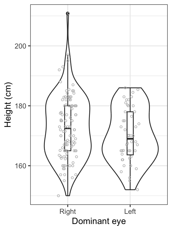
Figure 14.4: Violin and boxplot of the heights of students with right (n = 106) and left (n = 48) dominant eyes. Boxes delimit the first to third quartiles, bold lines represent the group medians, and whiskers extend to 1.5 times the IQR. Points beyond whiskers are extreme observations.
Interpretation
We can see in the preceding figure that heights are generally similar between students with left dominant eyes and those with right dominant eyes. However, it appears that the spread of the heights is greater among students with right dominant eyes. We will need to be careful about the equal-variance assumption for the 2-sample t-test.
14.3.4 Assumptions of the 2-sample t-test
The assumptions of the 2-sample t-test are as follows:
- each of the two samples is a random sample from its population
- the numerical variable is normally distributed in each population
- the variance (and thus standard deviation) of the numerical variable is the same in both populations
Test for normality
Now let’s check the normality assumption by plotting a normal quantile plot for each group.
We’ll introduce the facet_grid function that enables plotting of side-by-side panels according to a grouping variable.
students %>%
  ggplot(aes(sample = height_cm)) +
  stat_qq(shape = 1, size = 2) +
  stat_qq_line() +
  facet_grid(~ Dominant_eye) +
  xlab("Normal quantile") +
  ylab("Height (cm)") +
  theme_bw()
Figure 14.5: Normal quantile plots of height for students with right (n = 106) or left (n = 48) dominant eyes.
A reasonable statement would be:
“The normal quantile plots show that student height is generally normally distributed for students with left or right dominant eyes. There is one observation among the right-dominant eye students that is a bit off the line.”
Test for equal variances
Now we need to test the assumption of equal variance among the groups, using Levene’s Test as we learned in the checking assumptions tutorial.
## Levene's Test for Homogeneity of Variance (center = median)
##        Df F value Pr(>F)
## group   1   0.907 0.3424
##       152
It uses a test statistic “F”, and we see here that the P-value associated with the test statistic is larger than 0.05, so we don’t reject the implied null hypothesis that the variances are equal.
We state “A Levene’s test showed no evidence against the assumption of equal variance (F = 0.91; P-value = 0.342).”
Thus, we’ll proceed with conducting the 2-sample t-test.
14.3.5 Conduct the 2-sample t-test
We use the t.test function again for this test.
height.ttest <- students %>%
  t.test(height_cm ~ Dominant_eye,
         data = ., var.equal = TRUE, conf.level = 0.95)
The only difference from the implementation used in the paired t-test is:
- we include the “var.equal = TRUE” argument
We again include the argument “data = .”, which tells the t.test function that whatever data was passed to it from the preceding line is what will be used
We’ll learn a bit later what to due when the equal variance assumption is not met.
Let’s look at the result:
##
##  Two Sample t-test
##
## data:  height_cm by Dominant_eye
## t = 1.6, df = 152, p-value = 0.1117
## alternative hypothesis: true difference in means between group Right and group Left is not equal to 0
## 95 percent confidence interval:
##  -0.6521529  6.2061545
## sample estimates:
## mean in group Right  mean in group Left
##            172.8368            170.0598
We see that the test produced a P-value greater than \(\alpha\), so we fail to reject the null hypothesis.
Note also that the output includes a confidence interval for the difference in group means. We need to include this in our concluding statement.
14.3.6 Concluding statement
Here’s an example of a concluding statement:
On average, students with left dominant eyes are similar in height to students with right dominant eyes (Figure 19.4) (2-sample t-test; t = 1.6; df = 152; P-value = 0.112; 95% confidence interval for the difference in height -0.652 \(< \mu_d <\) 6.206).