13.3 Confidence intervals for \(\mu\)
In an earlier tutorial we learned about the rule of thumb 95% confidence interval.
Now we will learn how to calculate confidence intervals more precisely.
There are two typical uses of confidence intervals:
- When we are estimating a population parameter (such as \(\mu\)) based on a random sample, in which case the confidence interval is an ideal measure of precision to accompany our estimate
- As an alternative to a formal hypothesis test, in which case we determine whether the hypothesized value of the population parameter (e.g. \(\mu_0\)) is a plausible value for \(\mu\), based on the confidence interval calculated using our sample data
We’ll explore the latter use of confidence intervals later in this tutorial. For now, let’s demonstrate the first use of confidence intervals: as a measure of precision for an estimate.
13.3.1 Confidence interval as a measure of precision for an estimate
A straightforward way to calculate the confidence interval for the mean of a numeric variable is using the t.test function. For an example, see this tutorial section.
The formula for a 95% confidence interval for \(\mu\) is:
\[{\bar{Y}} - t_{0.05(2),df}SE_{\bar{Y}} < \mu < {\bar{Y}} + t_{0.05(2),df}SE_{\bar{Y}}\]
The \(t_{0.05(2),df}\) represents the critical value of t for a two-tailed test with \(\alpha = 0.05\), and degrees of freedom (df), which is calculated from our sample size as \(df = n - 1\).
\(SE_{\bar{Y}}\) is the familiar standard error of the mean, calculated as:
\[SE_{\bar{Y}} = \frac{s}{\sqrt{n}}\]
The lower 95 confidence limit is the value to the left of the \(\mu\) in the equation above, and the upper 95% confidence limit is the value to the right of of the \(\mu\) in the equation.
So now we need to figure out the critical value \(t_{0.05(2),df}\).
For the body temperature example, we have \(n = 25\) and thus \(df = 25-1 = 24\).
Optionally, we could assign all these values to objects first, for use later:
The function we use to find the critical value of t is the base function qt:
?qtThe qt function only deals with one tail of the distribution. Thus, if we have a two-sided alternative hypothesis, we need to divide our \(\alpha\) level by two in order to calculate the appropriate critical value of t.
The following graph illustrates this for the t distribution associated with df = 24 and \(\alpha(2)\) = 0.05. Specifically, the \(t_{crit}\) values are shown by the vertical lines, and delimit the points beyond which the area under the curve towards the tail is equal to \(\alpha / 2\) (and thus the total area of both red zones= \(\alpha\)).
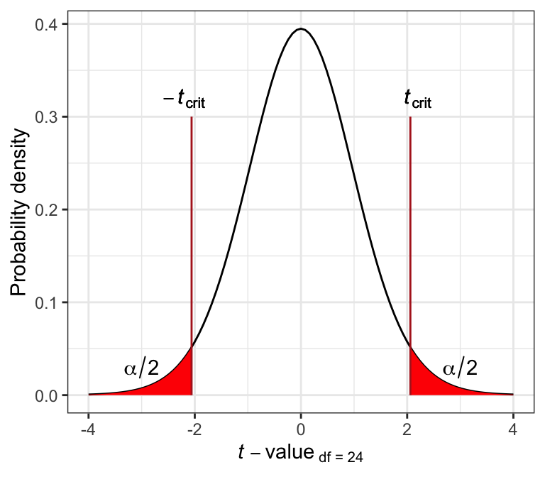
Figure 13.2: The t distribution for df = 24.
Here’s the code to calculate the critical value of t, and recall that we’ve defined alpha and d_f above:
In the code above:
- We assign the result to a new object called
tcrit - The \(\alpha(2) = 0.05\) is divided by 2, because we have a two-sided alternative hypothesis
- The degrees of freedom (which we stored in an object called
d_f) - We specified
lower.tail = FALSEto tell R that we’d like to focus on calculating the critical value for the right-hand (upper) tail, and thus the positive critical value
Alternatively, we could simply provide the values of alpha and degrees of freedom directly to the function arguments:
TIP
If instead we wanted to calculate a 99% confidence interval, then \(\alpha(2) = 0.01\), and we’d use 0.01 instead of 0.05 in the qt function above. Try it out!
Now let’s see what the output is:
## [1] 2.063899So to recap, this procedure used R code to give us what we’d otherwise need to look up in a statistical table, like the one provided in the text book.
Now that we’ve determined the value for \(t_{0.05(2),24}\), we need to calculate \(SE_{\bar{Y}}\), which we already learned how to do. So let’s improve on what we learned in the estimation tutorial, where we learned how to calculate the rule-of-thumb confidence interval.
There, we generated a table (actually a “tibble”) of summary statistics that included the rule-of-thumb confidence limits; now we can include the precisely calculated lower and upper 95% confidence limits.
Recall that we’ve already created an object “tcrit” that holds our required critical value of t.
Here we’ll assign the output to a tibble called “bodytemp.stats”:
bodytemp.stats <- bodytemp %>%
  summarise(
    Count = n() - naniar::n_miss(temperature),
    Mean_temp = mean(temperature, na.rm = TRUE),
    SD_temp = sd(temperature, na.rm = TRUE),
    SEM = SD_temp/sqrt(Count),
    Lower_95_CL = Mean_temp - tcrit * SEM,
    Upper_95_CL = Mean_temp + tcrit * SEM
  )
The summarise function is used to create new summary variables, as we’ve learned before.
The new part here is that we’re calculating precisely the lower and upper 95% confidence limits, using the combination of the tcrit value that we calculated and the “SEM” (standard error).
Now let’s use the kable function to produce a nice table, and here we’ll use “digits = 3” because that’s appropriate for the confidence limits (noting that it will report three decimal places for all our calculated values):
| Count | Mean_temp | SD_temp | SEM | Lower_95_CL | Upper_95_CL |
|---|---|---|---|---|---|
| 25 | 98.524 | 0.678 | 0.136 | 98.244 | 98.804 |
If we wanted to report the confidence interval on its own, we can get the necessary information from our newly created tibble “bodytemp.stats”, and type the following inline code in our markdown text (NOT in a code chunk):

Figure 13.3: Example of inline markdown and R code for a confidence interval
Which will provide:
98.244 < \(\mu\) < 98.804
13.3.2 Confidence interval approach to hypothesis testing
Recall our null and alternative hypotheses for the body temperature example:
H0: The mean human body temperature is 98.6\(^\circ\)F (\(\mu_0\) = 98.6\(^\circ\)F).
HA: The mean human body temperature is not 98.6\(^\circ\)F (\(\mu_0 \ne 98.6^\circ\)F).
The null hypothesis proposed \(\mu_0\) = 98.6\(^\circ\)F.
The confidence interval approach to testing a null hypothesis involves:
- specifying a level of confidence, 100% \(\times\) (1-\(\alpha\)), such as 95%
- calculating the confidence interval for \(\mu\) using the sample data
- determining whether or not \(\mu_0\) lies within the calculated confidence interval
If it does, then the proposed value of \(\mu_0\) is plausible, and there’s no reason to reject the null hypothesis.
If it does not, then we reject the null hypothesis and conclude that plausible values of \(\mu\) are between our lower and upper confidence limits.
For example, for the body temperature example, we calculated a 95% confidence interval as:
98.244 < \(\mu\) < 98.804
The hypothesized value of \(\mu_0\) was 98.6\(^\circ\)F, which is encompassed by our confidence interval. Thus, it is a plausible value, and there is no reason to reject the null hypothesis.
- Practice confidence intervals
- First, using the
bodytempdataset, calculate the 99% confidence interval for the mean body temperature in the population.
- Then, using the “stalkies” dataset, use the confidence interval approach (95% confidence) to test the hypothesis that the average eye span in the population is \(\mu_0\) = 8.1mm