11.3 Binomial distribution
The binomial distribution provides the probability distribution for the number of “successes” in a fixed number of independent trials, when the probability of success is the same in each trial.
Here’s the formula:
It turns out there’s a handy function dbinom (available in the base R package) that will calculate the exact probability associated with any particular outcome for a random trial with a given sample space (set of outcomes) and probability of success. It uses the equation shown above.
Check the help file for the function:
?dbinomDice example
Imagine rolling a fair, 6-sided die n = 6 times (six random trials). Let’s consider rolling a “4” a “success”.
What is the probability of observing two fours (i.e. two successes) in our 6 rolls of the die (random trials)?
We have X = 2 (the number of successes), p = 1/6 (the probability of a success in each trial), and n = 6 (the number of trials).
Here’s the code, where “x” represents our “X”, “size” represents the number of trials (“n”), and “prob” is the probability of success in each trial (here, 1/6).
We’ll create an object to hold the number of trials we wish to use first:
## [1] 0.2009388Thus, the probability of rolling two fours (i.e. having 2 successes) out of 6 rolls of the dice is about 0.201.
In order to get the probabilities associated with each possible outcome (i.e. 0 through 6 successes), we use the code shown in the chunk below.
exact.probs.6 <- tibble(
  X = 0:num.trials,
  probs = dbinom(x = 0:num.trials, size = num.trials, prob = 1/6)
  )
exact.probs.6
## # A tibble: 7 × 2
## X probs
## <int> <dbl>
## 1 0 0.3349
## 2 1 0.4019
## 3 2 0.2009
## 4 3 0.05358
## 5 4 0.008038
## 6 5 0.0006430
## 7 6 0.00002143Above we created a new tibble object (using the function tibble) called “exact.probs.6”, with a variable “X” that holds each of the possible outcomes (X = 0 through 6 or the number of trials), and “probs” that holds the probability of each outcome, calculated using the dbinom function:
See that the dbinom function will accept a vector of values of x, for which the associated probabilities are calculated.
Now let’s use these exact probabilities to create a barplot showing an exact, discrete probability distribution, corresponding to the binomial distribution with a sample size (number of trials) of n = 6 and a probability of success p = 1/6:
ggplot(exact.probs.6, aes(y = probs, x = X)) +
  geom_bar(stat = "identity", fill = "lightgrey", colour = "black") +
  xlab("Number of successes (X)") +
  ylab("Pr[X]") +
  theme_bw()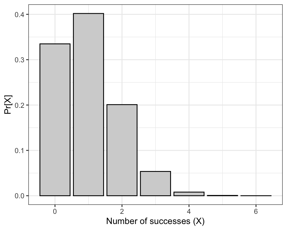
Figure 11.1: Probability of obtaining X successes out of 6 random trials, with probability of success = 1/6.
What if we wished to calculate the probability of getting at least two fours in our 6 rolls of the dice?
Consult the bar chart above. Recall that “rolling a 4” is our definition of a “success” (it could have been “rolling a 1”, or “rolling a 5” - these all result in the same calculation). Thus to calculate the probability of getting at least 2 successes we need to sum up the probabilities associated with getting 2, 3, 4, 5, and 6 successes.
We can do this using the following R code:
## [1] 0.2632245Note that we ask the dbinom function to do the calculation for each of the 2:num.trials outcomes of interest. We store these calculated probabilities in a new object “probs.2_to_6”.
Then, we use the sum function to sum up the probabilities within that object.
The resulting value of 0.2632245 looks about right based on our bar chart!
Now let’s increase the number of trials to n = 15, and compare the distribution to that observed using n = 6:
num.trials <- 15
exact.probs.15 <- tibble(
  X = 0:num.trials,
  probs = dbinom(x = 0:num.trials, size = num.trials, prob = 1/6)
  )
exact.probs.15
## # A tibble: 16 × 2
## X probs
## <int> <dbl>
## 1 0 6.491e- 2
## 2 1 1.947e- 1
## 3 2 2.726e- 1
## 4 3 2.363e- 1
## 5 4 1.418e- 1
## 6 5 6.237e- 2
## 7 6 2.079e- 2
## 8 7 5.346e- 3
## 9 8 1.069e- 3
## 10 9 1.663e- 4
## 11 10 1.996e- 5
## 12 11 1.814e- 6
## 13 12 1.210e- 7
## 14 13 5.583e- 9
## 15 14 1.595e-10
## 16 15 2.127e-12Now plot the binomial probability distribution:
ggplot(exact.probs.15, aes(y = probs, x = X)) +
  geom_bar(stat = "identity", fill = "lightgrey", colour = "black") +
  xlab("Number of successes (X)") +
  ylab("Pr[X]") +
  theme_bw()
Figure 11.2: Probability of obtaining X successes out of 15 random trials, with probability of success = 1/6.
- Challenge: Binomial probabilities
- Use the
dbinomfunction to calculate the probability of rolling three “2”s when rolling a fair six-sided die 20 times. - Produce a graph of a discrete probability distribution for this scenario: p = 1/4, and n = 12.