13.2 One-sample t-test
We previously learned statistical tests for testing hypotheses about categorical response variables. For instance, we learned how to conduct a \(\chi^2\) contingency test to test the null hypothesis that there is no association between two categorical variables.
Here we are going to learn our first statistical test for testing hypotheses about a numeric response variable, specifically one whose probability distribution in the population is normally distributed.
13.2.1 Hypothesis statement
Review the earlier tutorial that lists the steps to hypothesis testing.
We’ll use the body temperature data for this example, as described in example 11.3 in the text.
Americans are taught as kids that the normal human body temperature is 98.6 degrees Farenheit.
Are the data consistent with this assertion?
- We’ll use a one-sample t-test test to test the null hypothesis, because we’re dealing with a single numerical response variable, and we’re using a sample of individuals to draw inferences about a hypothesized (population) mean \(\mu_0\)
The hypotheses for this test:
H0: The mean human body temperature is 98.6\(^\circ\)F (\(\mu_0\) = 98.6\(^\circ\)F).
HA: The mean human body temperature is not 98.6\(^\circ\)F (\(\mu_0 \ne 98.6^\circ\)F).
TIP
You can add a degree symbol using this syntax in markdown: $^\circ$, so degrees Celsius would be $^\circ$C
- We’ll use an \(\alpha\) level of 0.05.
- It is a two-tailed alternative hypothesis
13.2.2 Assumptions of one-sample t-test
The assumptions of the one-sample t-test are as follows:
- the sampling units are randomly sampled from the population (a standard assumption)
- the variable is normally distributed in the population
Consult the “checking assumptions” tutorial for how to formally check the second assumption. For now we’ll assume both assumptions are met.
If the normal distribution assumption is not met, and no data transformation helps, then one can conduct a “non-parametric” test in lieu of the one-sample t-test, including a “Sign test” or a “Wilcoxon signed-rank test”. A tutorial on non-parametric tests is under development, but will not be deployed until 2023. Consult chapter 13 in the Whitlock & Schluter text, and this website for some R examples.
13.2.3 A graph to accompany a one-sample t-test
Let’s create a histogram of the body temperatures, because this is the most appropriate way to visualize the frequency distribution of a single numeric variable.
Histograms may look a little wonky if you have small sample sizes. This is OK!
If you forget how to create a histogram, consult the previous tutorial on visualizing a single numeric variable.
Here we’ll learn a few more tricks for producing a high-quality histogram.
The first step is to figure out the minimum and maximum values of your numeric variable, and you should have already done this when using the skim_without_charts function to get an overview of the dataset (when you first imported the data).
For the temperature variable, our minimum and maximum values were 97.4 and 100, respectively.
We’ll use this information to ensure that the histogram spans the appropriate range along the x-axis, and to decide on the appropriate “bin widths”:
bodytemp %>%
  ggplot(aes(x = temperature)) +
  geom_histogram(binwidth = 0.5, boundary = 97,
                 color = "black", fill = "lightgrey",) +
  xlab("Body temperature (degrees F)") +
  ylab("Frequency") +
  theme_bw()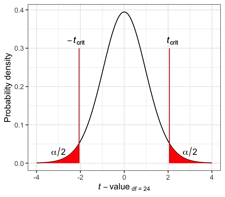
Figure 13.1: Frequency distribution of body temperature (degrees Farenheit) for 25 randomly chosen healthy people.
Notice the new argument to the geom_histogram function: “boundary”. Why include this? The minimum value in our dataset is 97.4. Based on our overview of the data, we decided to use a “binwidth” of 0.5. Therefore, it made most sense to have our bins (bars) start at 97, the first whole number preceding our minimum value, then have breaks every 0.5 units thereafter. Constructing the histogram this way makes it easier to interpret.
Recall that it can take a few times playing with different values of “binwidth” to make the histogram have the right number of bins.
Interpreting the histogram:
We can see in the histogram above that most of the individuals had temperatures between 98 and 99\(^\circ\)F, which is consistent with conventional wisdom, but there are 7 people with temperature below 98\(^\circ\)F, and 5 with temperatures above 99\(^\circ\)F. The frequency distribution is unimodal but not especially symmetrical.
13.2.4 Conduct the one-sample t-test
We use the t.test function (it comes with the base package loaded with R) to conduct a one-sample t-test.
?t.test This function is used for both one-sample and two-sample t-tests (covered later), and for calculating 95% confidence intervals for a mean (later in this tutorial).
Because this function has multiple purposes, be sure to pay attention to the arguments.
Here’s the code, which we’ll explain after:
body.ttest <- bodytemp %>%
  select(temperature) %>%
t.test(mu = 98.6, alternative = "two.sided", conf.level = 0.95) - We first assign our results to a new object called “body.ttest”
- We then
selectthe variable “temperature”, as this is the one being analyzed - We then conduct the test using the function
t.test, specifying the null hypothesized value as “mu = 98.6” - We specify “two.sided” for the “alternative” argument
- We provide the “conf.level” of 0.95, which is equal to \(1-\alpha\)
Let’s look at the results:
##
##  One Sample t-test
##
## data:  .
## t = -0.56065, df = 24, p-value = 0.5802
## alternative hypothesis: true mean is not equal to 98.6
## 95 percent confidence interval:
##  98.24422 98.80378
## sample estimates:
## mean of x
##    98.524
The output includes:
- The calculated test statistic t
- The degrees of freedom
- The P-value for the test
- A 95% confidence interval for \(\mu\)
- The sample-based estimate, denoted “mean of x”, but is our (\({\bar{Y}}\))
The observed P-value for our test is larger than our \(\alpha\) level of 0.05. We therefore fail to reject the null hypothesis.
13.2.5 Concluding statement for the one-sample t-test
Here’s an example of an appropriately worded concluding statement, including all the relevant information:
We have no reason to reject the null hypothesis that the mean body temperature of a healthy human is 98.6\(^\circ\)F (one-sample t-test; t = -0.56; n = 25 or df = 24; P = 0.58; 95% confidence interval: 98.244 \(< \mu <\) 98.804).
TIP
The confidence interval provided by the t.test function is accurate and good to report with your concluding statement for a one-sample t-test. However, below we learn a different way to calculate the confidence interval.