18.3 Making predictions

Even though the \(R^2\) value from our regression was rather low, we’ll proceed with using the model to make predictions.

It is not advisable to make predictions beyond the range of X-values upon which the regression was built. So in our case (see Figure 18.8), we would not wish to make predictions using species richness values beyond 16. Such “extrapolations” are inadvisable.

To make a prediction using our regression model, use the predict.lm function from the base stats package:

?predict.lm

If you do not provide new values of nSpecies (note that the variable name must be the same as was used when building the model), then it will simply use the old values that were supplied when building the regression model.

Here, let’s create a new tibble called “new.data” that includes new values of nSpecies (we’ll use 7 and 13 as example values) with which to make predictions:

new.data <- tibble(nSpecies = c(7, 13))

Now let’s make the predictions, and remember that these predicted values of biomass stability will be in the log scale:

predicted.values <- predict.lm(log.biomass.lm, newdata = new.data)
predicted.values

##        1        2 
## 1.428776 1.626331

Let’s superimpose these predicted values over the original scatterplot, using the annotate function from the ggplot2 package.

We re-use the code from our original geom_smooth plot above, and simply add the annotate line of code:

plantbiomass %>%
ggplot(aes(x = nSpecies, y = log.biomass)) +
  geom_point(shape = 1) +
  geom_smooth(method = "lm", colour = "black", 
              se = TRUE, level = 0.95) +
  annotate("point", x = new.data$nSpecies, y = predicted.values, shape = 2, size = 4) +
  xlab("Species richness") +
  ylab("Biomass stability") +
  theme_bw()

## `geom_smooth()` using formula = 'y ~ x'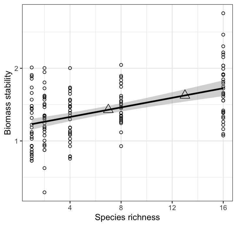

Figure 18.9: Stability of biomass production (log transformed) over 10 years in 161 plots and the initial number of plant species assigned to plots. Also shown are predicted values of stability across values of species richness.

As expected, Figure 18.9 shows the predicted values exactly where the regression line would be! We generally don’t present such a figure… here we’re just doing it for illustration.

18.3.1 Back-transforming regression predictions

The regression model we have calculated above is as follows:

ln(biomass stability) ~ 1.2 + 0.03(species richness)

Thus, any predictions we make are predictions of ln(y). It is sometimes desirable to report predicted values back in their original non-transformed state. To do this, follow the instructions in another tutorial dealing with data transformations.

---