17.3 Rank correlation (Spearman’s correlation)

If the assumption of bivariate normality is not met for Pearson correlation analysis, then we use Spearman rank correlation.

For example, if one or both of your numerical variables (X and / or Y) is actually a discrete, ordinal numerical variable to begin with (e.g. an attractiveness score that ranges from 1 to 5), then this automatically necessitates the use of Spearman rank correlation, because it does not meet the assumptions of bivariate normality. (This is why one needs to be careful with count data).

We’ll use the trick dataset for this example, and the data are described in example 16.5 in the text.

17.3.1 Hypothesis statements

The null and alternative hypotheses are:

H₀: There is no linear correlation between the ranks of the impressiveness scores and time elapsed until the writing of the description (\(\rho_{S} = 0\)).
H_A: There is a linear correlation between the ranks of the impressiveness scores and time elapsed until the writing of the description (\(\rho_{S} \ne 0\)).

Let’s use \(\alpha\) = 0.05.

As shown in the hypothesis statements above, we are interested in \(\rho_{S}\), which is the true correlation between the ranks of the variables in the population. We estimate this using \(r_{S}\), Spearman’s correlation coefficient.

Unlike in the Pearson correlation case (above), which uses t as a test statistic, the rank correlation analysis simply uses the actual Spearman correlation coefficient as the test statistic.

17.3.2 Visualize the data

Let’s visualize the association, again using the geom_jitter function to help see overlapping values:

trick %>%
  ggplot(aes(x = years, y = impressivenessScore)) +
  geom_jitter(shape = 1) +
  xlab("Years elapsed") +
  ylab("Impressiveness score") +
  theme_bw()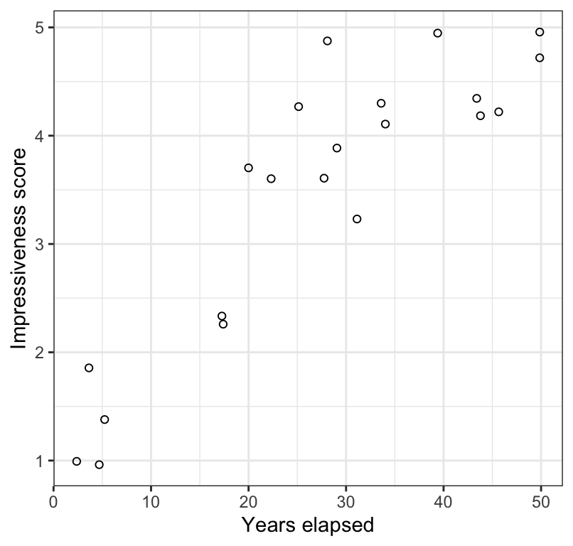

Figure 17.4: Scatterplot of the impressiveness of written accounts of the Indian rope trick by firsthand observers and the number of years elapsed between witnessing the event and writing the account (n = 21). Values have jittered slightly to improve legibility.

In Figure 17.4 we see a positive and moderately strong association between the impressiveness of written accounts of the Indian rope trick by firsthand observers and the number of years elapsed between witnessing the event and writing the account.

17.3.3 Assumptions of Spearman rank correlation

Spearman rank correlation assumes that:

• the observations are a random sample from the population
  
• the relationship between the two variables is monotonic; in other words it assumes that the relationship between the ranks of the two numerical variables is linear.

Checking assumptions

As in the Pearson correlation analysis, we use the scatterplot to check the assumptions.

As shown in Figure 17.4, there is a monotonic relationship between the two variables.

17.3.4 Conduct the test

We use the same cor.test function to conduct the test, but change the “method” argument accordingly:

trick.cor <- cor.test(x = trick$years, y = trick$impressivenessScore, 
                     method = "spearman", conf.level = 0.95,
                     alternative = "two.sided")

You may get a warning message, simply saying that it can’t compute exact P-values when there are ties in the ranked data. Don’t worry about this.

trick.cor.tidy <- trick.cor %>%
  broom::tidy()
trick.cor.tidy

## # A tibble: 1 × 5
##   estimate statistic    p.value method                          alternative
##      <dbl>     <dbl>      <dbl> <chr>                           <chr>      
## 1   0.7843     332.1 0.00002571 Spearman's rank correlation rho two.sided

• The “estimate” value represents the value of Spearman’s correlation coefficient \(r_S\); this is the value you report.
• The “statistic” value is NOT NEEDED so ignore
• The “p.value” associated with the observed Spearman’s correlation coefficient
• The “method” refers to the type of test conducted
• The “alternative” indicates whether the alternative hypothesis was one- or two-sided (the latter is the default)

There is no confidence interval reported with Spearman correlation analysis, so there is no need to report one in the concluding statement for a rank correlation. Nor is the degrees of freedom reported, so be sure to have figured out the appropriate degrees of freedom (or sample size “n”) to report in your concluding statement.

17.3.5 Concluding statement

As in the preceding Pearson correlation example, we can refer to the Figure in the parentheses of our concluding statement. Note also that we report n rather than degrees of freedom.

trick %>%
  ggplot(aes(x = years, y = impressivenessScore)) +
  geom_jitter(shape = 1) +
  xlab("Years elapsed") +
  ylab("Impressiveness score") +
  theme_bw()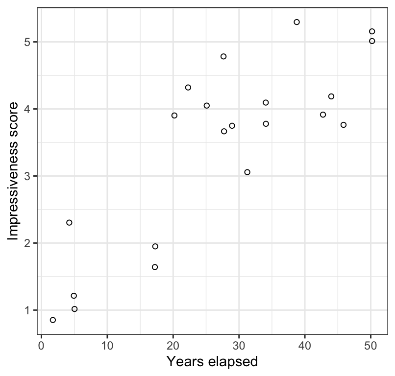

Figure 17.5: Scatterplot of the impressiveness of written accounts of the Indian rope trick by firsthand observers and the number of years elapsed between witnessing the event and writing the account (n = 21). Values have jittered slightly to improve legibility.

Concluding statement:

---

The rank of impressiveness scores of written accounts of the Indian rope trick by firsthand observers is significantly positively correlated with the rank of number of years elapsed between witnessing the event and writing the account (Figure 17.5; Spearman \(r_S\) = 0.78; \(n\) = 21; P < 0.001).

---