18.1 Load packages and import data

Load the tidyverse, skimr, broom, and knitr.

library(tidyverse)
library(skimr)
library(broom)
library(knitr)

We’ll use the “plantbiomass” dataset:

plantbiomass <- read_csv("https://raw.githubusercontent.com/ubco-biology/BIOL202/main/data/plantbiomass.csv")

## Rows: 161 Columns: 2
## ── Column specification ────────────────────────────────────────────────────────
## Delimiter: ","
## dbl (2): nSpecies, biomassStability
## 
## ℹ Use `spec()` to retrieve the full column specification for this data.
## ℹ Specify the column types or set `show_col_types = FALSE` to quiet this message.

The plantbiomass dataset (Example 17.3 in the text book) includes data describing plant biomass measured after 10 years within each of 5 experimental “species richness” treatments, wherein plants were grown in groups of 1, 2, 4, 8, or 16 species. The treatment variable is called nSpecies, and the response variable biomassStability is a measure of ecosystem stability. The research hypothesis was that increasing diversity (species richness) would lead to increased ecosystem stability.

Below is a visualization of the data.

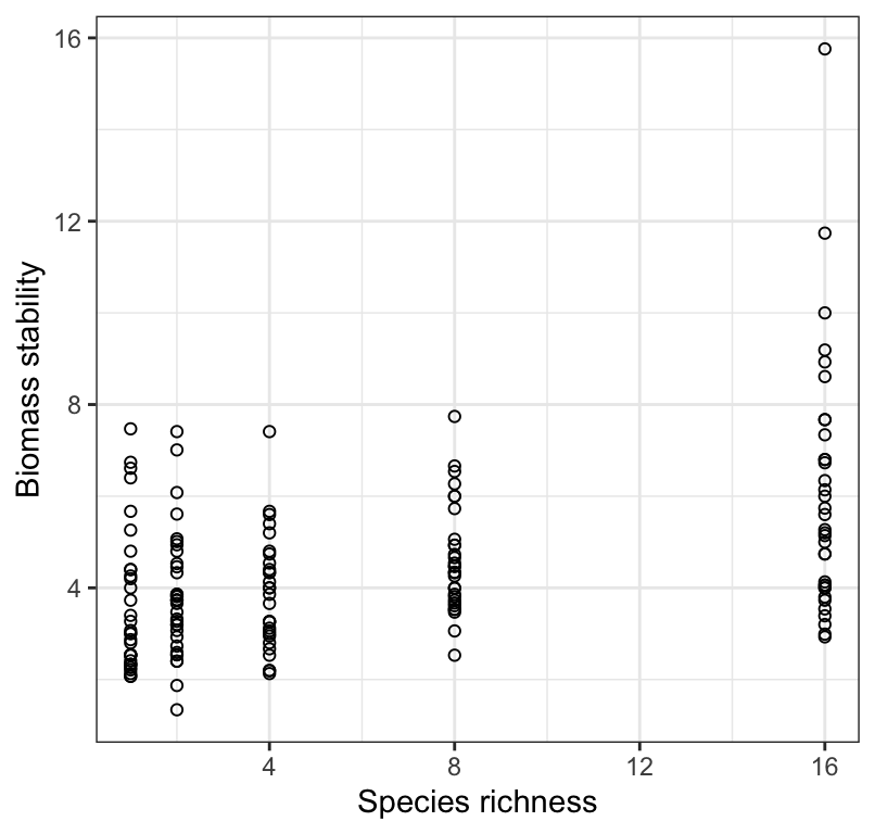
Figure 18.1: Stability of biomass production over 10 years in 161 plots and the initial number of plant species assigned to plots.

When one visualizes the data, one might ask why an ANOVA isn’t the analysis method of choice. If we were simply interested in testing the null hypothesis that “there is no difference in mean ecosystem stability among the species richness treatment groups”, then an ANOVA could be used, and we would simply treat the “species richness” variable as a categorical variable. However, here we are interested not simply in testing for differences among treatment groups, but more specifically in quantifying if and how ecosystem stability varies with variation in species richness, AND if so, whether we can reliably predict ecosystem stability based on species richness. For this, we need to construct a regression model.

Let’s have a look at the data:

plantbiomass %>% skim_without_charts()

(#tab:view_data_lsr)Data summary

Name	Piped data
Number of rows	161
Number of columns	2
_______________________
Column type frequency:
numeric	2
________________________
Group variables	None

Variable type: numeric

skim_variable	n_missing	complete_rate	mean	sd	p0	p25	p50	p75	p100
nSpecies	0	1	6.32	5.64	1.00	2.00	4	8.0	16.00
biomassStability	0	1	4.42	1.95	1.34	3.07	4	5.2	15.76

We see that both variables are numeric, and that there are 161 observations overall.

---