12.5 \(\chi\)² Contingency Test

When the contingency table is of dimensions greater than 2 x 2, the most commonly applied test is the \(\chi\)² Contingency Test.

For this activity we’re using the “worm” data associated with Example 9.4 on page 244 of the test. Please read the example!

---

12.5.1 Hypothesis statement

As shown in the text example, we have a 2 x 3 contingency table, and we’re testing for an association between two categorical variables.

Here are the null and alternative hypotheses (compare these to what’s written in the text):

H₀: There is no association between the level of trematode parasitism and the frequency (or probability) of being eaten.
H_A: There is an association between the level of trematode parasitism and the frequency (or probability) of being eaten.

• We use \(\alpha\) = 0.05.
  
• It is a two-tailed alternative hypothesis
  
• We’ll use a contingency test to test the null hypothesis, because this is appropriate for analyzing for association between two categorical variables, and when the resulting contingency table has dimension greater than 2 x 2.
  
• We will use the \(\chi\)² test statistic, with degrees of freedom equal to (r-1)(c-1), where “r” is the number of rows, and “c” is the number of colums, so (2-1)(3-1) = 2.
  
• We must check assumptions of the \(\chi\)² contingency test
• It is always a good idea to present a figure to accompany your analysis; in the case of a contingency test, the figure heading will include information about the sample size / total number of observations

---

12.5.2 Display the contingency table

Let’s generate a contingency table:

worm %>%
  tabyl(fate, infection) %>%
  adorn_totals(where = c("row", "col"))

##       fate highly lightly uninfected Total
##      eaten     37      10          1    48
##  not eaten      9      35         49    93
##      Total     46      45         50   141

Hmm, the ordering of the categories of the categorical (factor) variable “infection” is the opposite to what is displayed in the text.

TIP The ordering of the categories is not actually crucial to this type of analysis, but it’s certainly better practice to show them in appropriate order!

In order to change the order of categories in a character variable, here’s what you do (consult this resource for additional info).

First, convert the character variable to a “factor” variable as follows:

worm$infection <- as.factor(worm$infection)

Now check the default ordering of the levels using the levels function (it should be alphabetical):

levels(worm$infection)

## [1] "highly"     "lightly"    "uninfected"

Now change the ordering as follows:

worm$infection <- factor(worm$infection, levels = c("uninfected", "lightly", "highly"))
levels(worm$infection)

## [1] "uninfected" "lightly"    "highly"

Now re-display the contingency table, first storing it in an object “worm.table”:

worm.table <- worm %>%
  tabyl(fate, infection) %>%
  adorn_totals(where = c("row", "col"))
worm.table

##       fate uninfected lightly highly Total
##      eaten          1      10     37    48
##  not eaten         49      35      9    93
##      Total         50      45     46   141

That’s better!

Visualize it nicely with kable:

kable(worm.table)

fate	uninfected	lightly	highly	Total
eaten	1	10	37	48
not eaten	49	35	9	93
Total	50	45	46	141

12.5.3 Visualize a mosaic plot

Here’s a mosaic plot with an ideal figure caption included:

worm %>%
    ggplot() +
    geom_mosaic(aes(x = product(infection), fill = fate)) +
    scale_fill_manual(values=c("darkred", "gold")) +
    scale_y_continuous(breaks = seq(0, 1, by = 0.2)) +
    xlab("Level of infection") +
    ylab("Relative frequency") +
    theme_bw()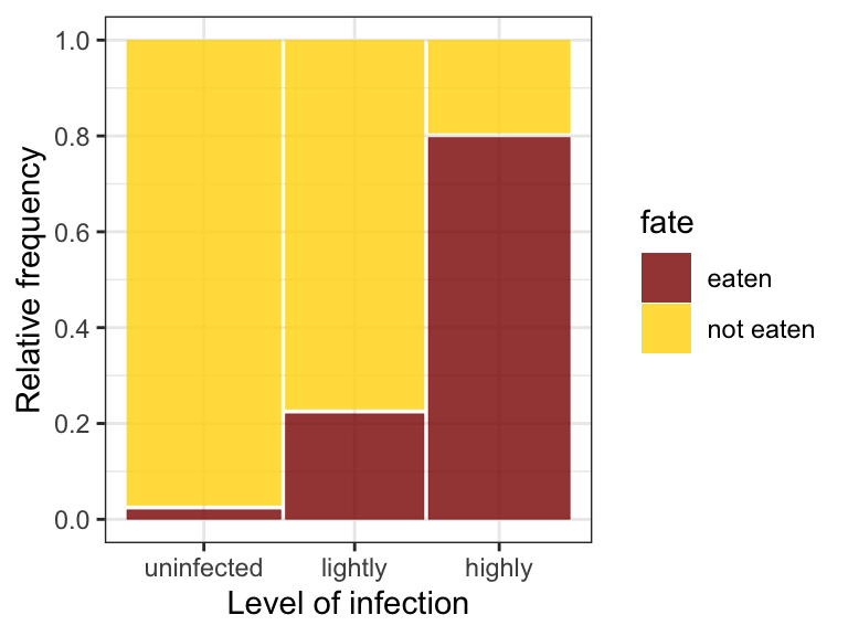

Figure 12.2: Mosaic plot of bird predation on killifish having different levels of trematode parasitism. A total of 50, 45, and 46 fish were in the uninfected, lightly infected, and highly infected groups.

In the code above we manually specified the two fill colours using the scale_fill_manual function.

12.5.4 Check the assumptions

The \(\chi\)² contingency test (also known as association test) has assumptions that must be checked prior to proceeding:

• none of the categories should have an expected frequency of less than one
• no more than 20% of the categories should have expected frequencies less than five

To test these assumptions, we need to actually conduct the test, because in doing so R calculates the expected frequencies for us.

Conduct the test using the chisq.test function from janitor package. NOTE this again overlaps with a function name from the base R package, so we’ll need to specify that we want the “janitor” version of the function.

We need our contingency table as input to the function, but this time without margin totals.

We’ll assign the results to an object “worm.chisq.results”:

worm.chisq.results <- worm %>%
    tabyl(fate, infection) %>%
    janitor::chisq.test()

Have a look at the output:

worm.chisq.results

## 
##  Pearson's Chi-squared test
## 
## data:  .
## X-squared = 69.756, df = 2, p-value = 7.124e-16

Although only a few bits of information are provided here, the object actually contains a lot more information.

Don’t try getting an overview of the object using our usual skim_without_charts approach.. that won’t work.

Instead, simply use this code:

names(worm.chisq.results)

## [1] "statistic" "parameter" "p.value"   "method"    "data.name" "observed" 
## [7] "expected"  "residuals" "stdres"

As you can see, one of the names is expected. This is what holds our expected frequencies (and note that these values do not need to be whole numbers, unlike the observed frequencies):

kable(worm.chisq.results$expected)

	fate	uninfected	lightly	highly
eaten	eaten	17.02128	15.31915	15.65957
not eaten	not eaten	32.97872	29.68085	30.34043

We see that all our assumptions are met: none of the cells (cross-classified categories) in the table have an expected frequency of less than one, and no more than 20% of the cells have expected frequencies less than five.

12.5.5 Get the results of the test

We can see the results of the \(\chi\)² test by simply typing the name of the results object:

worm.chisq.results

## 
##  Pearson's Chi-squared test
## 
## data:  .
## X-squared = 69.756, df = 2, p-value = 7.124e-16

This shows a very large value of \(\chi\)² (69.76) and a very small P-value - much smaller than our stated \(\alpha\). So we reject the null hypothesis.

Concluding statement

The probability of being eaten is significantly associated with the level of trematode parasitism (\(\chi\)² contingency test; df = 2; \(\chi\)² = 69.76; P < 0.001). Based on our mosaic plot (Fig. X), the probability of being eaten increases substantially with increasing intensity of parasitism.