15.1 The Basic Graph

The following assumes you’re using R and RMarkdown.

Install the libraries if needed

install.packages("ggplot2")
install.packages("palmerpenguins")

Load them

library(ggplot2) # for graphics
library(palmerpenguins) # penguins data set

## 
## Attaching package: 'palmerpenguins'

## The following objects are masked from 'package:datasets':
## 
##     penguins, penguins_raw

First, make sure we know a bit about our data set

head(penguins)

## # A tibble: 6 × 8
##   species island    bill_length_mm bill_depth_mm flipper_length_mm body_mass_g
##   <fct>   <fct>              <dbl>         <dbl>             <int>       <int>
## 1 Adelie  Torgersen           39.1          18.7               181        3750
## 2 Adelie  Torgersen           39.5          17.4               186        3800
## 3 Adelie  Torgersen           40.3          18                 195        3250
## 4 Adelie  Torgersen           NA            NA                  NA          NA
## 5 Adelie  Torgersen           36.7          19.3               193        3450
## 6 Adelie  Torgersen           39.3          20.6               190        3650
## # ℹ 2 more variables: sex <fct>, year <int>

Next, we call ggplot, define our data set, and then the variables to plot on the x and y axes:

ggplot(data = penguins, aes(x = sex, y = body_mass_g))

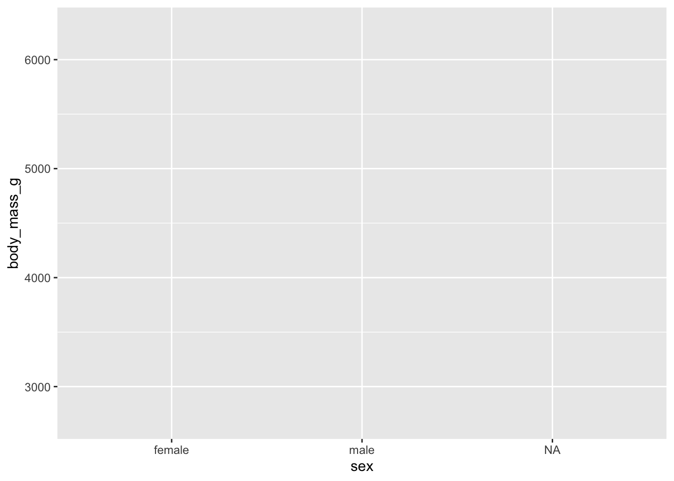
This sets us up with a blank grid with x and y axis ticks corresponding to your variable values and x and y axis labels corresponding to your variables.

Now we call a plot type to represent our data, in this case, a box plot

ggplot(data = penguins, aes(x = sex, y = body_mass_g)) +
  geom_boxplot()

## Warning: Removed 2 rows containing non-finite outside the scale range
## (`stat_boxplot()`).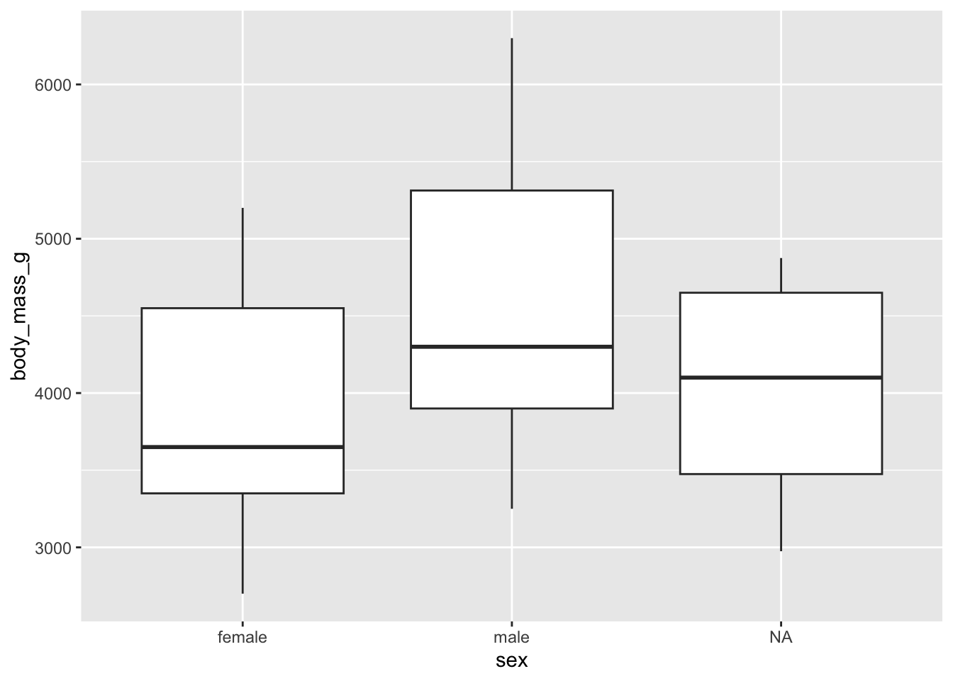

We have some NA values in our data set. We won’t worry about cleaning those up here. But we will suppress the error message with a code chunk option.

```{r, warning = FALSE}
ggplot(data = penguins, aes(x = sex, y = body_mass_g)) +
  geom_boxplot()
```

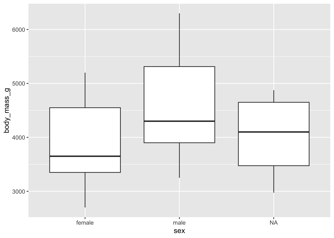
Chunk options are independent of ggplot itself and impact the knitting process of your RMarkdown document. For a more detailed overview of the code chunks options available to you, check out Xie Yihuis page on Knitr chunk options.