Using the RScripts
R scripts are text files containing the commands (aka code) and comments used to perform computations. For BIOL 205, we’ve written the majority of the code for you. In BIOL 202, you’ll be doing much more of this from scratch. Even though much of the code has been written for you, we encourage you to read through the scripts in detail and see if you can figure out with the help of the comments exactly what’s going on!
There is a separate R script for each type of variable combination you might have for your research project. When it comes time for your final analysis, download the R script that corresponds to the types of variables you have in your experiment. In the mean time, download all or any that you’re interested in looking through.
- Both response and explanatory variables are categorical
- Both response and explanatory variables are quantitative
- Categorical explanatory variable and quantitative response variable
While there are instructions within the R scripts themselves, the following sections describe how to use the R scripts in more detail. Be sure to read everything here and in the R scripts!
Alongside each line of code in the script is a comment proceeded with a hash tag (#). The comments are either descriptions of what the code is doing or instructions describing things you need to do.
You must correctly set up your project and working directory using the instructions below for this to work. You must also not simply open your R script, but instead launch your RProject file and then from within RStudio load the script from the built in file manager.
The general workflow here is:
- Launch RStudio using your RPoject file
- Load your data
- Provide the script with your variable names and the labels you’d like to use on your graphs
- Generate a graph; the script will save these to your
figures/directory - Run your descriptive stats; the script will save these to your
report/directory where you can copy the relevant information to your RMarkdown file - Run you statistical analyses; the script will save these to your
report/directory where you can copy the relevant information to your RMarkdown file
If you quite RStudio, you will need to re-run steps 1-3 to do any of steps 4-6 again.
Step 1: Set your working directory
If you haven’t already, make sure your working directory is set according to the instructions here in the Procedures and Guidelines Document.
Your directory should look something like this when you’re done, that is, after downloading at least one script, ensuring your data is in the project’s data folder, you’ve created an RMarkdown file, you’ve generated an RPoject file and put everything in its respective directory. Don’t worry if you don’t have all these things ready yet, just make sure that when you’re ready to run your scripts with your data, this is the model you’re working with.
├── BIOL205_RP/
│   ├── BIOL205_report.RProj
│   ├── data/
│   │   ├── 20221023_sample-data.csv
│   ├── figures/
│   ├── report/
│   │   ├── 20220101_Lab03_205_Assignment_V1.Rmd
│   ├── scripts/
│   │   ├── BIOL205_Script_Quantitative-Categorical.R
Step 2: Installing & Loading Required Packages
We’ll be using a couple of features that are not part of the basic install of R in our scripts. We add additional features in R with packages.
Packages in R contain a set of functions, code, and data that you can use for your analysis. Before you can use the functions within a package, the package must be both installed in R, which we do once, and loaded into R, which we do each time we start the application.
While packages only need to be installed once, if you're on a lab computer, since the computers are re-set at the end of each day you may need to re-install packages at each log in.
To install packages noted in the R script, copy the installation lines of code without the preceding hashtag (#) ie. remove the # from
# install.packages("ggplot2")so it looks like this
install.packages("ggplot2")and copy it into the R console (lower left pane of RStudio). When you hit enter on your keyboard the package will install. Be sure to do this for all of the required packages noted in the R script; these are in the first few lines of each script.
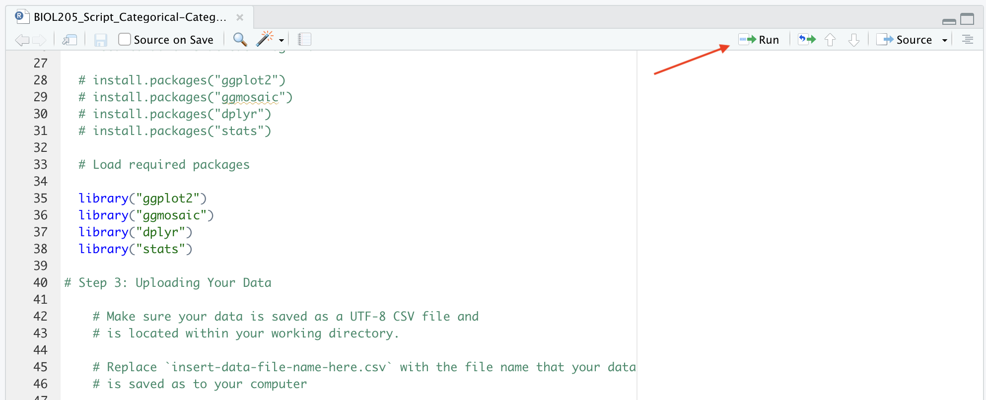
Once packages are installed, they must be loaded to your current session. You will have to do this each time you re-start R. To load packages use the library() function by running the lines of code pre-written into your R script. For example, run library(ggplot2) by placing your cursor in that line of code and clicking the ‘Run’ button at the top right of the working document. To load all packages at the same time, use your cursor to highlight all of the sections of code you want to run (lines 35-38 in the screenshot below), and then click ‘run’.
Running code can be done several ways in RStudio. You can go through line by line, putting you cursor in the line you wish to run, and executing each independently of the next. Or you can run a section of code by highlighting the ‘chunk’ you want to run.
The scripts are broken into ‘steps’. It’s probably best to highlight whole sections of each step and then running that chunk. But if you’d like to run line by line to get a better sense of what’s happening, go for it!
To quickly run a line of code, place your cursor on the line and use ctrl + Enter or Command + Enter if you’re on a Mac.
Step 3: Uploading your data
Replace the content within the quotes that read ‘insert-data-file-name-here.csv’ with the file name that your data is saved as to your computer. This will be in between lines 45 and 50 depending on the script you’re using.
If my data file was called 20221023_sample-data.csv, I’d change the following line
my_file <- paste0(dir,"insert-data-file-name-here.csv") # assign file name to a variableto
my_file <- paste0(dir,"20221023_sample-data.csv") # assign file name to a variableIf your data file contains a header row, be sure that the following line, which reads
my_data <- read.csv(file = my_file, header = TRUE)shows header = TRUE. If you have no header row, simply change the code to header = FALSE.
Step 4: Visualizing your data
You'll need to tell R some information before you can create graphs or do analyses. Specifically, you need to assign the names of your variables and axis labels. You can do this by
- Replacing “X variable name” and “Y variable name” with the names of your x and y variables
- Replacing “X label name” and “Y label name” with your desired x and y axes labels
So, we update the following lines
x_var <- "X variable name" # Replace with the name of your x variable
x_label <- "X label name" # Replace with your desired x axis label
y_var <- "Y variable name" # Replace with the name of your x variable
y_label <- "Y label name" # Replace with your desired y axis label
with something like
x_var <- "ht" # Replace with the name of your x variable
x_label <- "Height (in cm)" # Replace with your desired x axis label
y_var <- "day" # Replace with the name of your x variable
y_label <- "Day" # Replace with your desired y axis label
R is case sensitive. When providing your variable names, make sure they match exactly the variables used in your csv file!
In the R script for a categorical explanatory and a categorical response variable, code for both a boxplot and a stripchart is included.
Recall that according to the Biology Procedures and Guidelines document, you should use a boxplot if the groups of your categorical variable have more than 20 data points. Alternatively, you should use a stripchart if each group contains less than 20 data points. Be sure to only produce one desired figure.
In some of the R scripts there are some additional pieces of code that you don’t need to worry about for now; you’ll learn more about these in BIOL 202!
For example, we have to factor the categorical variables before producing graphs. You will see this additional code if the script you are using includes categorical variables.
In the code for creating a boxplot or stripchart, we refer to a function that calculates confidence intervals. So we have to define that function prior to running the code to produce the figure. You will find this additional piece of code in your R script if your experiment has a categorical explanatory variable and quantitative response variable.
There are some regions in the R scripts where variables are re-named or manipulated. If your up for it, take some time to read through the script and see if you can figure out exactly what’s happening!
Now you’re ready to run the code to create your figures and statistical calculations! Remember, once the code has been run, your figures will show in the lower right panel of RStudio under ‘Plots’ as well as being exported as .png image to your figures/ directory, and the results of your statistical analyses will be displayed in your R console, the lower left panel, as well as being saved as either .csv or .txt to your reports/ directory.
Step 5: Calculate descriptive statistics
The code here should run smoothly if everything in the proceeding steps was done correctly. Once the code has been run, your descriptive statistics will be printed in the console of RStudio (lower left panel). The instructions below describe how to interpret this output depending on the types of variables in your experiment.
Two Categorical Variables
Here is an example of the descriptive statistics output produced by the R script for two categorical variables. The explanatory (independent) variable and its associated groups appear in the first column, while the response (dependent) variable appears at the top. In this case the explanatory variable was species and the response variable was sex. The numbers provided in the table describe the frequency for each category. For example, in this sample there was 1 female Adelie penguin and 0 male Chinstrap penguins.
##            sex
## species     female male
##   Adelie        73   73
##   Chinstrap     34   34
##   Gentoo        58   61
Two Quantitative Variables
Here is an example of the output produced by the R script for two quantitative variables. The explanatory (independent) variable appears in the first row, while the response (dependent) variable appears in the second row. n indicates the sample size, while the following columns represent the mean, standard deviation, median, and interquartile range, respectively.
##                  n mean   sd median  iqr
## bill_length_mm 344 43.9 5.46     NA 9.27
## bill_depth_mm  344 17.2 1.97     NA 3.10
One Categorical and One Quantitative Variable
Here is an example of the output produced by the R script for one categorical and one quantitative variable. This table is organized so that the descriptive statistics of the quantitative response variable are reported based on the groups of the explanatory variable. n indicates the sample size, while the following columns represent the mean, standard deviation, median, and interquartile range, respectively. For example, the mean mass (g) for Adelie penguins in this sample is 3775 g.
##     species   n   mean     sd median   iqr
## 1    Adelie 152 3700.7 458.57   3700 650.0
## 2 Chinstrap  68 3733.1 384.34   3700 462.5
## 3    Gentoo 124 5076.0 504.12   5000 800.0
Take a screenshot of these values or write them down for writing your lab report later.
Step 6: Performing statistical analyses
Similar to with the descriptive statistics, the code here should run smoothly if everything in the proceeding steps was done correctly. The type of statistical analyses you will perform depends on the types of variables in your experiment.
Code for all possible statistical tests is included within the R scripts. Only run the code that corresponds with the type of variables in your experiment. Use the guidelines below to help you choose the appropriate statistical test.
Both response (dependent) and explanatory (independent) variables are categorical
- Both your response and explanatory variables have exactly 2 groups -> Use Fisher’s Exact Test
- At least one of your response or explanatory variables has more than 2 groups -> Use Chi-Square Contingency Analysis
Both response (dependent) and explanatory (independent) variables are quantitative
- Use Correlation Analysis
Response (dependent) variable is quantitative and explanatory (independent) variable is categorical
- Your categorical variable has exactly 2 groups -> Use Two Sample T-test
- Your categorical variable has more than 2 groups -> Use ANOVA
When interpreting the output from a statistical analysis for this project, focus on the p-value provided by R. You’ll learn more about the other details shown by the output in BIOL 202! Below are some examples of output for each type of statistical test.
Penguins data set with sex and species variables - the p-value is evident:
##
##  Fisher's Exact Test for Count Data
##
## data:  fisher.table
## p-value = 0.979
## alternative hypothesis: two.sided
Chi-Square Contingency Analysis
Penguins data set with sex and species variables - the p-value is evident:
##
##  Pearson's Chi-squared test
##
## data:  chi.table
## X-squared = 0.048607, df = 2, p-value = 0.976Penguins data set with bill_length_mm and bill_depth_mm variables - the p-value is fairly evident, labeled p.value:
## # A tibble: 1 × 8
## estimate statistic p.value parameter conf.low conf.high method alter…¹
## <dbl> <dbl> <dbl> <int> <dbl> <dbl> <chr> <chr>
## 1 -0.235 -4.46 0.0000112 340 -0.333 -0.132 Pearson's p… two.si…
## # … with abbreviated variable name ¹alternativePenguins data set with species - filtered to Chinstrap and Adelie - and body_mass_g variables - the p-value is evident:
##
##  Two Sample t-test
##
## data:  body_mass_g by species
## t = -0.50809, df = 217, p-value = 0.6119
## alternative hypothesis: true difference in means between group Adelie and group Chinstrap is not equal to 0
## 95 percent confidence interval:
##  -158.21193   93.35996
## sample estimates:
##    mean in group Adelie mean in group Chinstrap
## 3700.662 3733.088Penguins data set with species and body_mass_g variables - the p-value is under the header Pr(>F):
## Analysis of Variance Table
##
## Response: body_mass_g
##            Df    Sum Sq  Mean Sq F value    Pr(>F)
## species     2 146864214 73432107  343.63 < 2.2e-16 ***
## Residuals 339  72443483   213698
## ---
## Signif. codes:  0 '***' 0.001 '**' 0.01 '*' 0.05 '.' 0.1 ' ' 1