6 Describing a single variable

Tutorial learning objectives

In this tutorial you will:

Learn how to calculate the main descriptor of a categorical variable: the proportion
Learn how to calculate measures of centre and spread for a single numerical variable

6.1 Load packages and import data

Let’s load some packages first:

library(dplyr)
library(ggplot2)
library(readr)
library(palmerpenguins)
library(knitr)
library(janitor)
library(biol202)

We will use the following datasets in this tutorial:

the birds dataset contains counts of different categories of bird observed at a marsh habitat
the penguins dataset that is available as part of the palmerpenguins package

data(birds)

6.2 Describing a categorical variable

The proportion is the most important descriptive statistic for a categorical variable. It measures the fraction of observations in a given category within a categorical variable.

For example, the birds dataset has a single variable called type that includes tallies (frequencies) of each of four categories of bird observed at a marsh habitat.

birds
#> # A tibble: 86 × 1
#>    type     
#>    <fct>    
#>  1 Waterfowl
#>  2 Predatory
#>  3 Predatory
#>  4 Waterfowl
#>  5 Shorebird
#>  6 Waterfowl
#>  7 Waterfowl
#>  8 Songbird 
#>  9 Predatory
#> 10 Waterfowl
#> # ℹ 76 more rows

The proportion of birds belonging to a given category is the same as the relative frequency of birds belonging to a given category.

In a previous tutorial, using the tigerdeaths dataset, we learned how to create a frequency table that included relative frequencies.

Let’s use the same approach for the birds dataset. First we create the frequency table, then we display the table with an appropriate heading:

birds.table <- birds %>%
  count(type, sort = TRUE) %>% 
  mutate(relative_frequency = n / sum(n)) %>% 
  adorn_totals()

Note

NOTE If there are missing values (“NA”) in the categorical variable, the preceding code will successfully enumerate those and create an “NA” category in the frequency table.

Now display the table:


birds.table %>%
  kable(caption = "Frequency table showing the frequencies of each of four types of bird observed at a marsh habitat (N = 86)", digits = 3)

Table 6.1: Frequency table showing the frequencies of each of four types of bird observed at a marsh habitat (N = 86)

type	n	relative_frequency
Waterfowl	43	0.500
Predatory	29	0.337
Shorebird	8	0.093
Songbird	6	0.070
Total	86	1.000

We can see, for example, that the proportion (relative frequency) of birds belonging to the “Predatory” category was 0.3372093.

We calculate proportions (relative frequencies) using the simple formula:

\[\hat{p} = \frac{n_i}{N}\] Where \[n_i\] is the frequency of observations in the given category of interest i, and N is total number of observations (sample size) across all categories.

Note

Reminder Proportions, and thus relative frequencies, must be between 0 and 1.

6.3 Describing a numerical variable

Numeric variables are described with measures of centre and spread.

Before calculating descriptive statistics for a numeric variable, it is advisable to visualize its frequency distribution first. Why? Because characteristics of the frequency distribution will govern which measures of centre and spread are more reliable or representative.

If the frequency distribution is roughly symmetric and does not have any obvious outliers, then the mean and the standard deviation are the preferred measures of centre and spread, respectively
If the frequency distribution is asymmetric and / or has outliers, the median and the inter-quartile range (IQR) are the preferred measures of centre and spread

It is often the case, however, that all four measures are presented together.

Note

New tool Introducing the summarise function.

The dplyr package has a handy summarise (equivalently summarize) function for calculating descriptive statistics.

Check out its help file by copying the following code into your command console:

?summarise

Let’s use the penguins dataset for our demonstrations.

The first step is to visualize the frequency distribution. Given that this is a numeric variable, we do this using a histogram, as we learned in a previous tutorial.


ggplot(data = penguins, aes(x = body_mass_g)) +
  geom_histogram(binwidth = 500, colour = "black", fill = "lightgrey") +
  xlab("Body mass (g)") +
  ylab("Frequency") +
  theme_bw()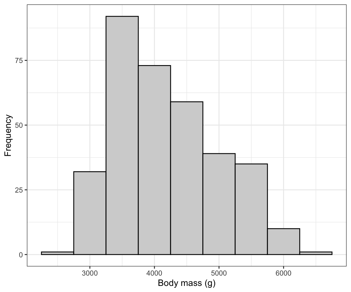

Figure 6.1: Histogram of body mass (g) for 342 penguins

We are reminded that the distribution of body mass is moderately positively skewed and thus asymmetric, with a single mode near 3500g. There are no obvious outliers in the distribution.

This means that the median and IQR should be the preferred descriptors of centre and spread, respectively.

6.3.1 Calculating the median & IQR

So let’s calculate the median and IQR of body mass for all penguins. Let’s provide the code, then explain after:

penguins %>%
  summarise(
   median_body_mass_g =  median(body_mass_g),
   IQR_body_mass_g = IQR(body_mass_g)
    )

Uh oh! If you tried to run this code, it would have given you an error:

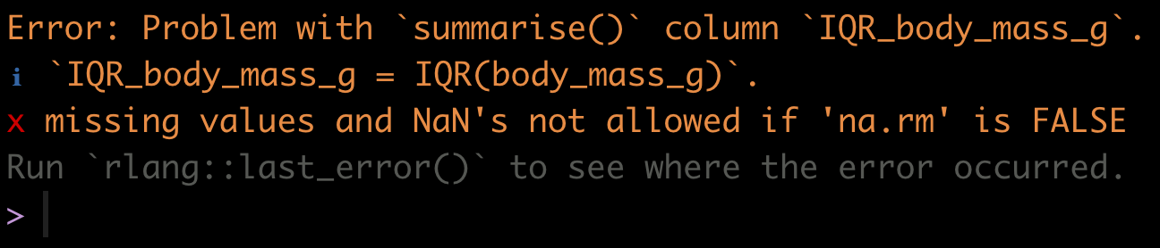
Figure 6.2: Error when functions encounter ‘NA’ values

We forgot that when we previously got an overview of the penguins dataset we discovered there were missing values (“NA” values)!

Note

TIP If there are “NA” values in the variable being analyzed, some R functions, such as the function median or mean, will simply return “NA”. To remedy this, we use the “na.rm = TRUE” argument.

Let’s try our code again, adding the “na.rm = TRUE” argument. And note that the key functions called within the summarise function are median and IQR (case sensitive!).

penguins %>%
  summarise(
   Median =  median(body_mass_g, na.rm = TRUE),
   InterQR = IQR(body_mass_g, na.rm = TRUE)
    )
#> # A tibble: 1 × 2
#>   Median InterQR
#>    <dbl>   <dbl>
#> 1   4050    1200

In the preceding code chunk, we have:

The name of the tibble (here penguins) being used in the subsequent functions
A pipe “%>% to tell R we’re not done coding
The summarise function (summarize will work too), telling R we’re going to calculate a new variable
The name we’ll give to the first variable we’re creating, here we call the variable “Median” (the “M” is capitalized to distinguish this variable name from the function median)
And we define how to calculate the “Median”, here using the median function
We feed the variable of interest from the penguins tibble, “body_mass_g”, to the median function, along with the argument “na.rm = TRUE”
We end the line with a comma, telling R that we’re not done providing arguments to the summarise function
We do the same for the inter-quartile range variable we’re creating called “InterQR”, calculating the value using the IQR function, and this time no comma at the end of the line, because this is the last argument being provided to the summarise function
We close out the parentheses for the summarise function

6.3.2 Calculating the mean & standard deviation

Although the median and IQR are the preferred descriptors for the body_mass_g variable, it is nonetheless commonplace to report the mean and standard deviation also.

Let’s do this, and while we’re at it, include even more descriptors to illustrate how they’re calculated.

This time we’ll put the output from our summarise function into a table, and then present it in a nice format, like we learned how to do for a frequency table.

Let’s create the table of descriptive statistics first, a tibble called “penguins.descriptors”, and we’ll describe what’s going on after (NOTE this code chunk was edited slightly on Sept. 30, 2021):

penguins.descriptors <- penguins %>%
  summarise( 
  Mean = mean(body_mass_g, na.rm = T),
  SD = sd(body_mass_g, na.rm = T),
  Median = median(body_mass_g, na.rm = T),
  InterQR = IQR(body_mass_g, na.rm = T),
  Count = sum(!is.na(body_mass_g)),
  Count_NA = sum(is.na(body_mass_g)))

The first 4 descriptive statistics are self-explanatory based on their variable names.

The last two: “Count” and “Count_NA” are providing the total number of complete observations in the body_mass_g variable (thus the number of observations that went into calculating the descriptive statistics), and then the total number of missing values (NAs) in the variable, respectively.

The last two lines of code above require further explanation:

This code: Count = sum(!is.na(body_mass_g)) counts the observations that are not missing. Reading it from the inside out:

is.na() asks of each value, “is this one missing?”, and returns TRUE or FALSE for each
the ! means not, so it flips those answers around: TRUE now marks every value that is present
sum() adds them up. R counts each TRUE as 1 and each FALSE as 0, so summing them counts the non-missing observations.

The same coding approach is used in the last line: Count_NA = sum(is.na(body_mass_g)). It is the same idea without the !, so it counts the values that are missing.

Note

This pair is worth committing to memory:

sum(!is.na(x)) — how many values of x are present
sum(is.na(x)) — how many are missing

You will use both all term. They use only base R, so they work anywhere, without loading any package.

Note

TIP It is important to calculate the total number of complete observations in the variable of interest, because, as described in the Biology Procedures and Guidelines document, this number needs to be reported in figure and table headings.

Now let’s show the table of descriptive statistics, using the kable function we learned about in a previous tutorial.


penguins.descriptors %>%
  kable(caption = "Descriptive statistics of measurements of body mass (g) for 342 penguins", digits = 3)

Table 6.2: Descriptive statistics of measurements of body mass (g) for 342 penguins

Mean	SD	Median	InterQR	Count	Count_NA
4201.754	801.955	4050	1200	342	2

Note

In another tutorial we’ll learn how to present the table following all the guidelines in the Biology Guidelines and Procedures document, including, for example, significant digits. For now, the preceding table is good!

Activity

Descriptive statistics: Create a histogram and table of descriptive statistics for the “flipper_length_mm” variable in the penguins dataset.

6.4 Describing a numerical variable grouped by a categorical variable

In this tutorial you’ll learn how to calculate descriptive statistics for a numerical variable grouped according to categories of a categorical variable.

For example, a common scenario in biology is to want to calculate and report the mean and standard deviation of a response variable for different “treatment groups” in an experiment. (More commonly we would report the mean and standard error, but that’s for a later tutorial!).

It is straightforward to modify the code we used in the preceding tutorial to do what we want.

Specifically, we use the group_by function from the dplyr package to tell R to do the calculations on the observations within each category of the grouping variable.

For example, let’s describe penguin body mass grouped by “species”.

We’ll create a new tibble object called “penguins.descriptors.byspecies”, and we insert one line of code using the group_by function, and telling R which categorical variable to use for the grouping (here, “species”):

penguins.descriptors.byspecies <- penguins %>%
  group_by(species) %>%
summarise(
  Mean = mean(body_mass_g, na.rm = T),
  SD = sd(body_mass_g, na.rm = T),
  Median = median(body_mass_g, na.rm = T),
  InterQR = IQR(body_mass_g, na.rm = T),
  Count = sum(!is.na(body_mass_g)),
  Count_NA = sum(is.na(body_mass_g)))

It’s that simple!

Let’s have a look at the output:

penguins.descriptors.byspecies
#> # A tibble: 3 × 7
#>   species    Mean    SD Median InterQR Count Count_NA
#>   <fct>     <dbl> <dbl>  <dbl>   <dbl> <int>    <int>
#> 1 Adelie    3701.  459.   3700    650    151        1
#> 2 Chinstrap 3733.  384.   3700    462.    68        0
#> 3 Gentoo    5076.  504.   5000    800    123        1

Activity

Use the kable function to output this new tibble in a nice format.